Deep equilibrium networks and their relation to system theory, part of the seminar Machine Learning in the Sciences by Mathias Niepert. The code for the examples shown is available on GitHub

Motivation

Equilibrium networks were introduced at NeurIPS 2019 with the main benefit being their memory efficiency. Compared to state-of-the-art networks deep equilibrium networks could reach the same level of accuracy without storing the output of each layer to do backpropagation. In this post, the goal is to stress the connection between deep equilibrium networks and how they can be applied to system identification and control. This link is also seen in a CDC 2022 and CDC 2021 paper.

To appreciate that connection let us assume an unknown nonlinear dynamical system that can be described by a discrete differential equation

with given initial condition $x^0$. The state is denoted by $x^k$, the input by $u^k$, and the output by $y^k$, the superscript indicates the time step of the sequence $k=1, \ldots, N$. The goal in system identification is to learn the functions $g_{\text{true}}: \mathbb{R}^{n_x} \times \mathbb{R}^{n_u} \mapsto \mathbb{R}^{n_y}$ and $f_{\text{true}}: \mathbb{R}^{n_x} \times \mathbb{R}^{n_u} \mapsto \mathbb{R}^{n_x}$ from a set of input-output measurements $\mathcal{D} = \lbrace (u, y)_i \rbrace$ for $i=1, \ldots, K$.

The system \eqref{eq:nl_system} maps an input sequence $u$ to an output sequence $y$, recurrent neural networks are a natural fit to model sequence-to-sequence maps. From a system theoretic perspective, recurrent neural networks are discrete, linear, time-invariant systems interconnected with a static nonlinearity known as the activation function, a very general formulation, therefore, follows as

with $w^k = \Delta(z^k)$. The standard recurrent neural network (See Equation 10 in Deep Learning Book Chapter 10) results as a special case of this more general description, this can be seen by choosing the hidden state $h^{k} = x^{k+1}$, $\Delta(z^k) = \tanh(z^k)$ and the following parameters:

Note that we neglected the bias terms.

The problem of learning the system \eqref{eq:nl_system} can now be made more formal. Given a dataset $\mathcal{D}$, find a parameter set $\theta = \lbrace A, B_1, B_2, C_1, D_{11}, D_{12}, C_2, D_{21}, D_{22} \rbrace$ such that the error between the prediction and the output measurement is small,

Before diving into deep equilibrium networks let us shortly recap the motivation. Recurrent neural networks are a good fit to model unknown dynamical systems. The parameters are tuned by looking at the difference between the prediction of the recurrent neural network and the output measurements. A more general description of a recurrent neural network is given by a general discrete, linear, time-invariant system interconnected with a static nonlinearity.

In the next section, the basic concept of deep equilibrium networks will be explained, this naturally leads to monotone operator equilibrium networks. We then come back to the motivation and the application of equilibrium networks for system identification.

The focus of this post is to highlight the link between deep equilibrium networks and their application in systems and control. Details on how to calculate the gradient and monotone operator theory are only referenced.

Deep equilibrium networks

Consider a input sequence $u$ that is fed through a neural network with $L$ layers, each layer $f_{\theta}^{[0]}(x^0, u), \ldots, f_{\theta}^{[L-1]}(x^{L-1}, u)$ contains different weights, where $x$ represents the hidden state and $f_{\theta}^{[i]}$ the activation function.

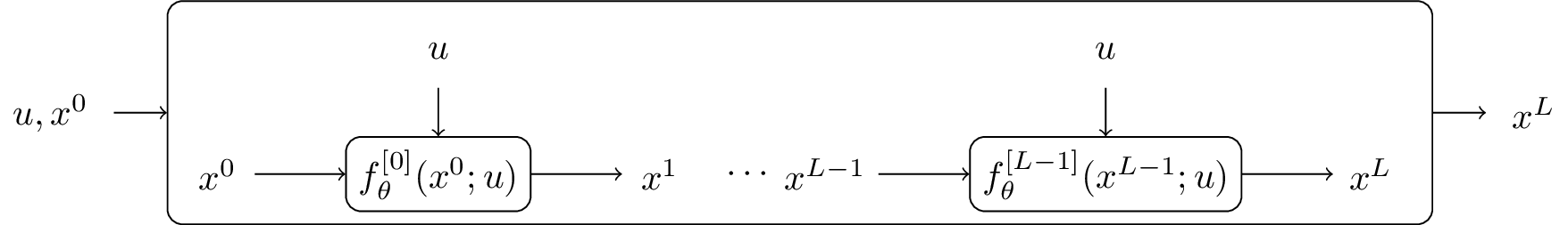
The first step towards deep equilibrium networks is to tie the weights $f_{\theta}^{[0]}(x^0, u) = f_{\theta}^{[i]}(x^0, u)$ for all $i=0, \ldots, L-1$. It turns out that this restriction does not hurt the prediction accuracy of the network, since any deep neural network can be replaced by a single layer by increasing the size of the weight (See Appendix C for details).

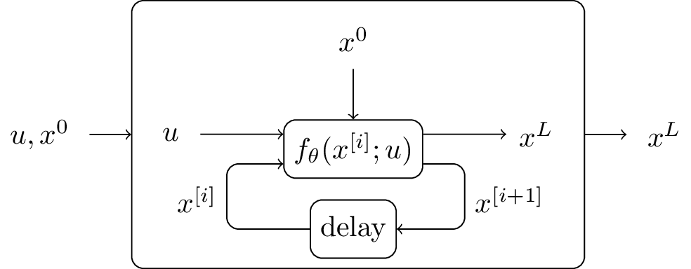
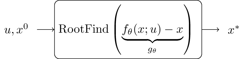
In the next step, the number of layers is increased $L \to \infty$. The forward pass can now also be formulated as finding a fixed point $x^{\star}$, which can be solved by several root fining algorithms as illustrated next.

Backward pass

To train the deep equilibrium network the gradient with respect to the parameters $\theta$ needs to be calculated from the forward pass. Traditionally this is achieved by stepping through the forward pass of the deep neural network. For deep equilibrium models however this is not desired, since the gradient should be independent of the root-finding algorithm.

The loss function follows as

with the output layer $h:\mathbb{R}^{n_z} \mapsto \mathbb{R}^{n_y}$, which can be any differentiable function (e.g. linear), $y$ is the ground-truth sequence and $\mathcal{L}:\mathbb{R}^{n_y}\times\mathbb{R}^{n_y} \mapsto \mathbb{R}$ is the loss function.

The gradient with respect to $(\cdot)$ (e.g. $\theta$) can now be calculated by implicit differentiation

were $J_{g_\theta}^{-1} \mid_{x^{\star}}$ is the inverse Jacobian of $g_{\theta}$ evaluated at $x^{\star}$

For details on the gradient and how it can be calculated see Chapter 4 of the implicit layer tutorial.

One major benefit of equilibrium networks is that no intermediate results on the forward pass needs to be stored, which reduces the memory complexity.

Example

Let us make a simple example to compare a fixed-layer neural network with a deep equilibrium model.

We assume:

• sequence length $T=3$
• the size of hidden state $n_x = 10$
• input and output size $n_y = n_u = 1$

The weights are randomly initialized and the initial hidden state is set to zero $x^0 = 0$, $W_h \in \mathbb{R}^{n_x \times n_x}$, $U_h\in \mathbb{R}^{n_x \times T}$ and we take a linear output layer with $W_y \in \mathbb{R}^{n_y \times n_x}$, the biases are accordingly.

The forward pass for $L$ layers sequence-to-sequence model in PyTorch:

# forward pass for fixed number of layers
x = torch.zeros(size=(1, n_x))
u = torch.tensor(u).reshape(1, n_u)
for l in range(L):
    x = nl(W_h(z) + U_h(u) + b_x)
y_hat = W_y(x) + b_y

The forward pass for the deep equilibrium model:

# DEQ
def g_theta(x):
    x = x.reshape(n_x,1)
    return np.squeeze(np.tanh(W_h_numpy @ z + U_h_numpy @ x + b_x_numpy) - z)

x_star, infodict, ier, mesg = fsolve(g_theta, x0=x_0, full_output=True)
x_star = z_star.reshape(n_z, 1)
y_hat_eq = W_y_numpy @ x_star + b_y_numpy

Note that the code is only small snippets that should give an idea of how to implement the models, the code is not supposed to run without further adjustment, for the root-finding algorithm scipy.optimize.fsolve is used.

The results for different values of $L$ are compared

Number of finite layers: 0       || x^{L-1} - x^{\star} ||^2: 0.7032
Number of finite layers: 1       || x^{L-1} - x^{\star} ||^2: 0.3898
Number of finite layers: 2       || x^{L-1} - x^{\star} ||^2: 0.2898
Number of finite layers: 3       || x^{L-1} - x^{\star} ||^2: 0.1621
Number of finite layers: 4       || x^{L-1} - x^{\star} ||^2: 0.09451
Number of finite layers: 10      || x^{L-1} - x^{\star} ||^2: 0.001685
Number of finite layers: 20      || x^{L-1} - x^{\star} ||^2: 7.595e-06
Number of finite layers: 30      || x^{L-1} - x^{\star} ||^2: 7.069e-08

The result shows that a feed-forward neural network converges to the same result as the equilibrium network if the layer size increases.

Monotone operator equilibrium networks

Looking at the results of the comparison a natural question to ask is whether the deep neural network always converges to a fixed point for sufficiently large $L$.

If the weight is initialized differently e.g. by a normal distribution with standard values mean=0, std=1.0 torch.nn.init.normal

W_h = torch.nn.Linear(in_features=n_z, out_features=n_z, bias=True)
torch.nn.init.normal_(W_h.weight)
U_h = torch.nn.Linear(in_features=n_x, out_features=n_z, bias=False)
W_y = torch.nn.Linear(in_features=n_z, out_features=n_x, bias=True)

The finite layer network reaches a different hidden state compared to the equilibrium network

    Number of finite layers: 0       || x^{L-1} - x^{\star} ||^2: 0.4664
    Number of finite layers: 1       || x^{L-1} - x^{\star} ||^2: 0.332
    Number of finite layers: 2       || x^{L-1} - x^{\star} ||^2: 1.035
    Number of finite layers: 3       || x^{L-1} - x^{\star} ||^2: 1.834
    Number of finite layers: 4       || x^{L-1} - x^{\star} ||^2: 2.348
    Number of finite layers: 10      || x^{L-1} - x^{\star} ||^2: 2.75
    Number of finite layers: 20      || x^{L-1} - x^{\star} ||^2: 2.724
    Number of finite layers: 30      || x^{L-1} - x^{\star} ||^2: 2.927

this can be seen by comparing the values for large $L$ values, where the state $x^{L-1}$ is not equal to the equilibrium state $x^{\star}$.

As an extension to deep equilibrium networks monotone operator equilibrium networks was introduced a year later at NeurIPS 2020. The monotone operator theory allows the formulation of constraints on the parameters that guarantee the existence and uniqueness of a fixed point. We refer to Appendix A of the original paper for an introduction to monotone operator theory. In this post, the monotone operator splitting technique is assumed to be one root-finding algorithm.

Consider (again) a weight-tied input-injected network

and an equilibrium point that remains constant after an update

Finding an equilibrium point of \eqref{eq:iter} is equivalent to finding a zero of the operator splitting problem $0 \in (F+G)(z^{\star})$ with the operators

and $\Delta(\cdot) = \operatorname{prox}_f^1(\cdot)$ for some convex closed proper function $f$, where $\operatorname{prox}_f^{\alpha}$ denotes the proximal operator

The monotone operator \eqref{eq:operator_splitting} is strongly monotone if

for $m>0$, this is equivalent to the existence and uniqueness of an equilibrium point $x^{\star}$.

For the scalar case, the monotonicity property is intuitive, consider

condition \eqref{eq:condition} refers to a positive slope for $F_{\text{scal}}(x)$

For details on the gradient we refer to the original publication and only mention that the gradient with respect to the parameters can be calculated by implicit differentiation.

Example

To see that condition \eqref{eq:condition} on the weight $W_h$, leads to a unique fixpoint, let us revisit our example for different initializations and print the eigenvalues of $(I-W_h)$:

min EW of (I-W_h): 0.6272        L: 40   || x^{L-1} - x^{\star} ||^2: 3.999e-08
min EW of (I-W_h): 0.3782        L: 40   || x^{L-1} - x^{\star} ||^2: 4.184e-08
min EW of (I-W_h): 0.5671        L: 40   || x^{L-1} - x^{\star} ||^2: 3.373e-08
min EW of (I-W_h): 0.6786        L: 40   || x^{L-1} - x^{\star} ||^2: 6.231e-08
min EW of (I-W_h): 0.8057        L: 40   || x^{L-1} - x^{\star} ||^2: 2.551e-08
min EW of (I-W_h): 0.662         L: 40   || x^{L-1} - x^{\star} ||^2: 3.364e-08
min EW of (I-W_h): 0.3946        L: 40   || x^{L-1} - x^{\star} ||^2: 4.522e-08
min EW of (I-W_h): 0.6532        L: 40   || x^{L-1} - x^{\star} ||^2: 2.656e-08
min EW of (I-W_h): 0.4264        L: 40   || x^{L-1} - x^{\star} ||^2: 3.059e-08
min EW of (I-W_h): 0.6787        L: 40   || x^{L-1} - x^{\star} ||^2: 5.395e-08

This supports the theoretical analysis.

System identification with equilibrium networks

The monotone operator equilibrium network guarantees the existence and uniqueness of a fixed point by introducing a constraint on the weight. This is achieved by only allowing parameters that satisfy the constraint \eqref{eq:condition}.

Now let us look back at the original problem of learning an unknown nonlinear differential equation \eqref{eq:nl_system} from a dataset $\mathcal{D}$ that consists of input-output measurements. How can we use equilibrium networks to improve prediction accuracy?

In the recurrent neural network, \eqref{eq:rnn_linear} the state that is fed through the nonlinear activation function $z^k$ depends on the output of the nonlinearity $w^k$ when the parameter $D_{22}$ is not zero. This is exactly a fixed point problem that needs to be solved before iterating through the sequence.

Before the equilibrium network where popular the parameter $D_{22}$ was usually set to zero to avoid such direct dependency between the output and the input. This reduced the expressiveness of the network \eqref{eq:rnn_linear}. Deep equilibrium networks allow for $D_{22}\neq 0$ to calculate the fixed point $z^{\star}$ in \eqref{eq:rnn_linear} and more important to calculate the gradient to adjust the parameters, monotone operator deep equilibrium networks even guarantee that $z^{\star}$ exists and that it is unique.

Additionally, and that is independent of deep equilibrium networks, the description of a recurrent neural network as a linear, time-invariant system with nonlinear disturbance as shown in \eqref{eq:rnn_linear} allows to use well-established theory of robust control to analyze stability and performance of the network.

Deep equilibrium networks (and monotone equilibrium networks) are interesting from a system theoretic view even though the successful applications are still missing, first promising results e.g. for identifying the vibration of an aircraft with performance guarantees are reported in Recurrent Equilibrium Networks: Unconstrained Learning of Stable and Robust Dynamical Models. The benefit of equilibrium network goes beyond memory efficiency.